import datetime
print(f"Last updated on {datetime.date.today()}.")

Last updated on 2026-03-15.

Demo script for the analyses done in Nakamura and Huang (2018, Science)

This is a complimentary demo script that can be used to implement the local wave activity, fluxes and flux convergence/divergence computation required in the analyses presented in Nakamura and Huang, Atmospheric Blocking as a Traffic Jam in the Jet Stream. Science. (2018)

This notebook demonstrate how to compute local wave activity and all the flux terms in equations (2) and (3) in NH2018 with the updated functionality in the python package falwa. To run the script, please install the package falwa using

python -m pip install .

after cloning the GitHub repo.

Please raise an issue in the GitHub repo or contact Clare S. Y. Huang (csyhuang@uchicago.edu) if you have any questions or suggestions regarding the package.

import datetime as dt
from math import pi
import numpy as np
from numpy import dtype
import xarray as xr
import matplotlib.pyplot as plt
%matplotlib inline
from falwa.oopinterface import QGFieldNH18
import falwa
print(falwa.__version__)

2.3.3

Load ERA-Interim reanalysis data retrieved from ECMWF server

The sample script in this directory download_example.py include the code to retrieve zonal wind field U, meridional wind field V and temperature field T at various pressure levels. Given that you have an account on ECMWF server and have the cdsapi package installed, you can run the scripts to download data from there:

python download_example.py

u_file = xr.open_dataset('2005-01-23_to_2005-01-30_u.nc')
v_file = xr.open_dataset('2005-01-23_to_2005-01-30_v.nc')
t_file = xr.open_dataset('2005-01-23_to_2005-01-30_t.nc')
ntimes = u_file.valid_time.size
time_array = u_file.valid_time

u_file

<xarray.Dataset>
Dimensions:         (valid_time: 32, pressure_level: 37, latitude: 121,
                     longitude: 240)
Coordinates:
    number          int64 ...
  * valid_time      (valid_time) datetime64[ns] 2005-01-23 ... 2005-01-30T18:...
  * pressure_level  (pressure_level) float64 1e+03 975.0 950.0 ... 3.0 2.0 1.0
  * latitude        (latitude) float64 90.0 88.5 87.0 85.5 ... -87.0 -88.5 -90.0
  * longitude       (longitude) float64 0.0 1.5 3.0 4.5 ... 355.5 357.0 358.5
    expver          (valid_time) <U4 ...
Data variables:
    u               (valid_time, pressure_level, latitude, longitude) float32 ...
Attributes:
    GRIB_centre:             ecmf
    GRIB_centreDescription:  European Centre for Medium-Range Weather Forecasts
    GRIB_subCentre:          0
    Conventions:             CF-1.7
    institution:             European Centre for Medium-Range Weather Forecasts
    history:                 2024-10-26T21:32 GRIB to CDM+CF via cfgrib-0.9.1...

xarray.Dataset

• Dimensions:
  • valid_time: 32
  • pressure_level: 37
  • latitude: 121
  • longitude: 240
• Coordinates: (6)
  • number
    ()
    int64
    ...

    long_name :

    ensemble member numerical id

    units :

    1

    standard_name :

    realization

    [1 values with dtype=int64]

  • valid_time
    (valid_time)
    datetime64[ns]
    2005-01-23 ... 2005-01-30T18:00:00

    long_name :

    time

    standard_name :

    time

    array(['2005-01-23T00:00:00.000000000', '2005-01-23T06:00:00.000000000',
           '2005-01-23T12:00:00.000000000', '2005-01-23T18:00:00.000000000',
           '2005-01-24T00:00:00.000000000', '2005-01-24T06:00:00.000000000',
           '2005-01-24T12:00:00.000000000', '2005-01-24T18:00:00.000000000',
           '2005-01-25T00:00:00.000000000', '2005-01-25T06:00:00.000000000',
           '2005-01-25T12:00:00.000000000', '2005-01-25T18:00:00.000000000',
           '2005-01-26T00:00:00.000000000', '2005-01-26T06:00:00.000000000',
           '2005-01-26T12:00:00.000000000', '2005-01-26T18:00:00.000000000',
           '2005-01-27T00:00:00.000000000', '2005-01-27T06:00:00.000000000',
           '2005-01-27T12:00:00.000000000', '2005-01-27T18:00:00.000000000',
           '2005-01-28T00:00:00.000000000', '2005-01-28T06:00:00.000000000',
           '2005-01-28T12:00:00.000000000', '2005-01-28T18:00:00.000000000',
           '2005-01-29T00:00:00.000000000', '2005-01-29T06:00:00.000000000',
           '2005-01-29T12:00:00.000000000', '2005-01-29T18:00:00.000000000',
           '2005-01-30T00:00:00.000000000', '2005-01-30T06:00:00.000000000',
           '2005-01-30T12:00:00.000000000', '2005-01-30T18:00:00.000000000'],
          dtype='datetime64[ns]')

  • pressure_level
    (pressure_level)
    float64
    1e+03 975.0 950.0 ... 3.0 2.0 1.0

    long_name :

    pressure

    units :

    hPa

    positive :

    down

    stored_direction :

    decreasing

    standard_name :

    air_pressure

    array([1000.,  975.,  950.,  925.,  900.,  875.,  850.,  825.,  800.,  775.,
            750.,  700.,  650.,  600.,  550.,  500.,  450.,  400.,  350.,  300.,
            250.,  225.,  200.,  175.,  150.,  125.,  100.,   70.,   50.,   30.,
             20.,   10.,    7.,    5.,    3.,    2.,    1.])

  • latitude
    (latitude)
    float64
    90.0 88.5 87.0 ... -88.5 -90.0

    units :

    degrees_north

    standard_name :

    latitude

    long_name :

    latitude

    stored_direction :

    decreasing

    array([ 90. ,  88.5,  87. ,  85.5,  84. ,  82.5,  81. ,  79.5,  78. ,  76.5,
            75. ,  73.5,  72. ,  70.5,  69. ,  67.5,  66. ,  64.5,  63. ,  61.5,
            60. ,  58.5,  57. ,  55.5,  54. ,  52.5,  51. ,  49.5,  48. ,  46.5,
            45. ,  43.5,  42. ,  40.5,  39. ,  37.5,  36. ,  34.5,  33. ,  31.5,
            30. ,  28.5,  27. ,  25.5,  24. ,  22.5,  21. ,  19.5,  18. ,  16.5,
            15. ,  13.5,  12. ,  10.5,   9. ,   7.5,   6. ,   4.5,   3. ,   1.5,
             0. ,  -1.5,  -3. ,  -4.5,  -6. ,  -7.5,  -9. , -10.5, -12. , -13.5,
           -15. , -16.5, -18. , -19.5, -21. , -22.5, -24. , -25.5, -27. , -28.5,
           -30. , -31.5, -33. , -34.5, -36. , -37.5, -39. , -40.5, -42. , -43.5,
           -45. , -46.5, -48. , -49.5, -51. , -52.5, -54. , -55.5, -57. , -58.5,
           -60. , -61.5, -63. , -64.5, -66. , -67.5, -69. , -70.5, -72. , -73.5,
           -75. , -76.5, -78. , -79.5, -81. , -82.5, -84. , -85.5, -87. , -88.5,
           -90. ])

  • longitude
    (longitude)
    float64
    0.0 1.5 3.0 ... 355.5 357.0 358.5

    units :

    degrees_east

    standard_name :

    longitude

    long_name :

    longitude

    array([  0. ,   1.5,   3. , ..., 355.5, 357. , 358.5])

  • expver
    (valid_time)
    <U4
    ...

    [32 values with dtype=<U4]

• Data variables: (1)
  • u
    (valid_time, pressure_level, latitude, longitude)
    float32
    ...

    GRIB_paramId :

    131

    GRIB_dataType :

    an

    GRIB_numberOfPoints :

    29040

    GRIB_typeOfLevel :

    isobaricInhPa

    GRIB_stepUnits :

    1

    GRIB_stepType :

    instant

    GRIB_gridType :

    regular_ll

    GRIB_uvRelativeToGrid :

    0

    GRIB_NV :

    0

    GRIB_Nx :

    240

    GRIB_Ny :

    121

    GRIB_cfName :

    eastward_wind

    GRIB_cfVarName :

    u

    GRIB_gridDefinitionDescription :

    Latitude/Longitude Grid

    GRIB_iDirectionIncrementInDegrees :

    1.5

    GRIB_iScansNegatively :

    0

    GRIB_jDirectionIncrementInDegrees :

    1.5

    GRIB_jPointsAreConsecutive :

    0

    GRIB_jScansPositively :

    0

    GRIB_latitudeOfFirstGridPointInDegrees :

    90.0

    GRIB_latitudeOfLastGridPointInDegrees :

    -90.0

    GRIB_longitudeOfFirstGridPointInDegrees :

    0.0

    GRIB_longitudeOfLastGridPointInDegrees :

    358.5

    GRIB_missingValue :

    3.4028234663852886e+38

    GRIB_name :

    U component of wind

    GRIB_shortName :

    u

    GRIB_totalNumber :

    0

    GRIB_units :

    m s**-1

    long_name :

    U component of wind

    units :

    m s**-1

    standard_name :

    eastward_wind

    [34383360 values with dtype=float32]

• Indexes: (4)
  • valid_time
    PandasIndex

    PandasIndex(DatetimeIndex(['2005-01-23 00:00:00', '2005-01-23 06:00:00',
                   '2005-01-23 12:00:00', '2005-01-23 18:00:00',
                   '2005-01-24 00:00:00', '2005-01-24 06:00:00',
                   '2005-01-24 12:00:00', '2005-01-24 18:00:00',
                   '2005-01-25 00:00:00', '2005-01-25 06:00:00',
                   '2005-01-25 12:00:00', '2005-01-25 18:00:00',
                   '2005-01-26 00:00:00', '2005-01-26 06:00:00',
                   '2005-01-26 12:00:00', '2005-01-26 18:00:00',
                   '2005-01-27 00:00:00', '2005-01-27 06:00:00',
                   '2005-01-27 12:00:00', '2005-01-27 18:00:00',
                   '2005-01-28 00:00:00', '2005-01-28 06:00:00',
                   '2005-01-28 12:00:00', '2005-01-28 18:00:00',
                   '2005-01-29 00:00:00', '2005-01-29 06:00:00',
                   '2005-01-29 12:00:00', '2005-01-29 18:00:00',
                   '2005-01-30 00:00:00', '2005-01-30 06:00:00',
                   '2005-01-30 12:00:00', '2005-01-30 18:00:00'],
                  dtype='datetime64[ns]', name='valid_time', freq=None))

  • pressure_level
    PandasIndex

    PandasIndex(Index([1000.0,  975.0,  950.0,  925.0,  900.0,  875.0,  850.0,  825.0,  800.0,
            775.0,  750.0,  700.0,  650.0,  600.0,  550.0,  500.0,  450.0,  400.0,
            350.0,  300.0,  250.0,  225.0,  200.0,  175.0,  150.0,  125.0,  100.0,
             70.0,   50.0,   30.0,   20.0,   10.0,    7.0,    5.0,    3.0,    2.0,
              1.0],
          dtype='float64', name='pressure_level'))

  • latitude
    PandasIndex

    PandasIndex(Index([ 90.0,  88.5,  87.0,  85.5,  84.0,  82.5,  81.0,  79.5,  78.0,  76.5,
           ...
           -76.5, -78.0, -79.5, -81.0, -82.5, -84.0, -85.5, -87.0, -88.5, -90.0],
          dtype='float64', name='latitude', length=121))

  • longitude
    PandasIndex

    PandasIndex(Index([  0.0,   1.5,   3.0,   4.5,   6.0,   7.5,   9.0,  10.5,  12.0,  13.5,
           ...
           345.0, 346.5, 348.0, 349.5, 351.0, 352.5, 354.0, 355.5, 357.0, 358.5],
          dtype='float64', name='longitude', length=240))

• Attributes: (6)

  GRIB_centre :

  ecmf

  GRIB_centreDescription :

  European Centre for Medium-Range Weather Forecasts

  GRIB_subCentre :

  0

  Conventions :

  CF-1.7

  institution :

  European Centre for Medium-Range Weather Forecasts

  history :

  2024-10-26T21:32 GRIB to CDM+CF via cfgrib-0.9.14.1/ecCodes-2.36.0 with {"source": "data.grib", "filter_by_keys": {"stream": ["oper"]}, "encode_cf": ["parameter", "time", "geography", "vertical"]}

Load the dimension arrays

In this version, the QGField object takes only: - latitude array in degree ascending order, and - pressure level in hPa in decending order (from ground to aloft).

xlon = u_file.longitude.values

# latitude has to be in ascending order
ylat = u_file.latitude.values
if np.diff(ylat)[0]<0:
    print('Flip ylat.')
    ylat = ylat[::-1]

# pressure level has to be in descending order (ascending height)
plev = u_file.pressure_level.values
if np.diff(plev)[0]>0:
    print('Flip plev.')
    plev = plev[::-1]

nlon = xlon.size
nlat = ylat.size
nlev = plev.size

Flip ylat.

clat = np.cos(np.deg2rad(ylat))     # cosine latitude
p0 = 1000.                          # surface pressure [hPa]
kmax = 49                           # number of grid points for vertical extrapolation (dimension of height)
dz = 1000.                          # differential height element
height = np.arange(0,kmax)*dz       # pseudoheight [m]
dphi = np.diff(ylat)[0]*pi/180.     # differential latitudinal element
dlambda = np.diff(xlon)[0]*pi/180.  # differential latitudinal element
hh = 7000.                          # scale height
cp = 1004.                          # heat capacity of dry air
rr = 287.                           # gas constant
omega = 7.29e-5                     # rotation rate of the earth
aa = 6.378e+6                       # earth radius
prefactor = np.array([np.exp(-z/hh) for z in height[1:]]).sum() # integrated sum of density from the level
                                                                #just above the ground (z=1km) to aloft
npart = nlat                        # number of partitions to construct the equivalent latitude grids
maxits = 100000                     # maximum number of iteration in the SOR solver to solve for reference state
tol = 1.e-5                         # tolerance that define convergence of solution
rjac = 0.95                         # spectral radius of the Jacobi iteration in the SOR solver.
jd = nlat//2+1                      # (one plus) index of latitude grid point with value 0 deg
                                    # This is to be input to fortran code. The index convention is different.

Set the level of pressure and the timestamp to display below

tstamp = [dt.datetime(2005,1,23,0,0) + dt.timedelta(seconds=6*3600) * tt for tt in range(ntimes)]
plev_selected = 10 # selected pressure level to display
tstep_selected = 0

Loop through the input file and plot computed quantities

for tstep in range(32):  # or ntimes

    uu = u_file.u.isel(valid_time=tstep).values[:, ::-1, :]
    vv = v_file.v.isel(valid_time=tstep).values[:, ::-1, :]
    tt = t_file.t.isel(valid_time=tstep).values[:, ::-1, :]

    qgfield_object = QGFieldNH18(xlon, ylat, plev, uu, vv, tt, northern_hemisphere_results_only=False)

    qgfield_object.interpolate_fields(return_named_tuple=False)

    qgfield_object.compute_reference_states(return_named_tuple=False)

    qgfield_object.compute_lwa_and_barotropic_fluxes(return_named_tuple=False)

    if tstep == tstep_selected:
        # === Below demonstrate another way to access the computed variables ===
        # 3D Variables that I would choose one pressure level to display
        variables_3d = [
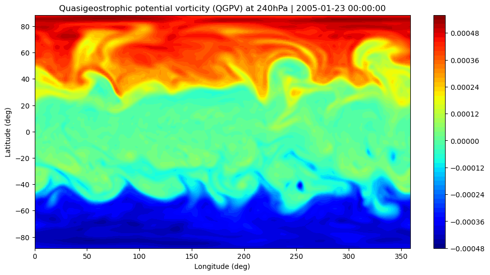
            (qgfield_object.qgpv, 'Quasigeostrophic potential vorticity (QGPV)'),
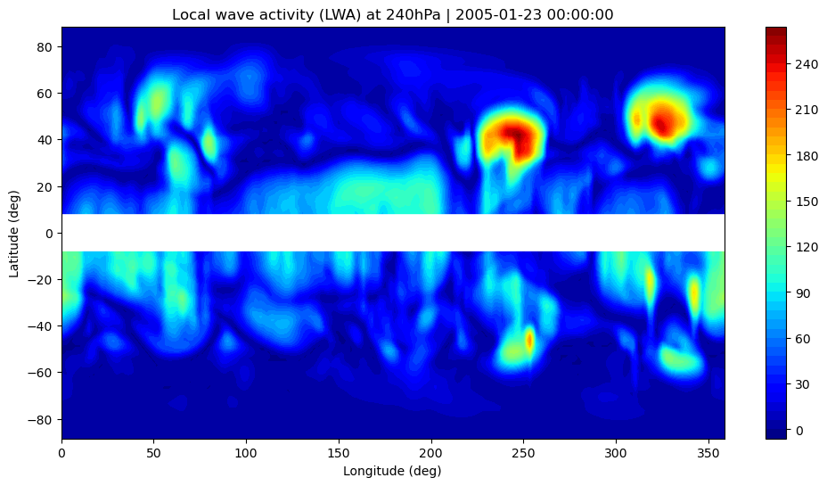
            (qgfield_object.lwa, 'Local wave activity (LWA)'),
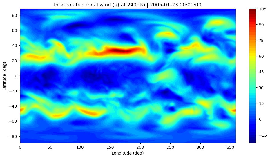
            (qgfield_object.interpolated_u, 'Interpolated zonal wind (u)'),
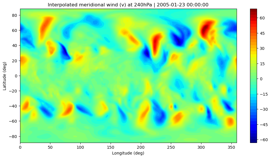
            (qgfield_object.interpolated_v, 'Interpolated meridional wind (v)')]

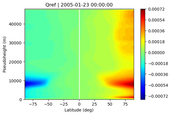
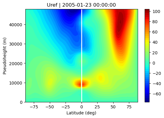
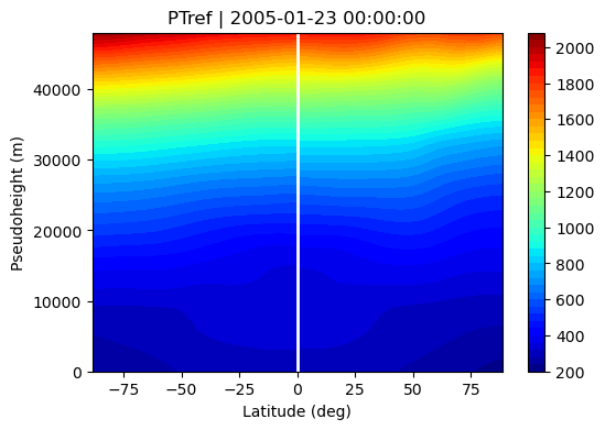
        # Reference states to be displayed on y-z plane
        variables_yz = [
            (qgfield_object.qref, 'Qref'),
            (qgfield_object.uref, 'Uref'),
            (qgfield_object.ptref, 'PTref')]

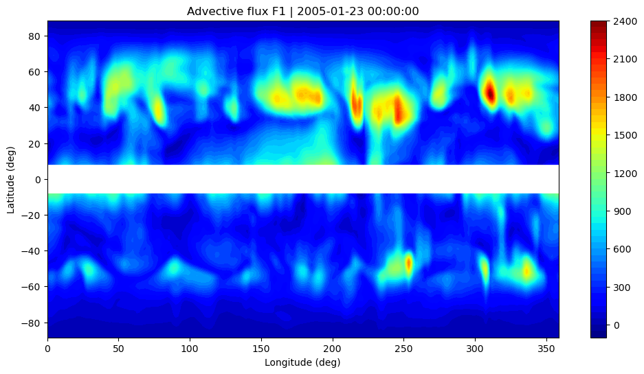
        # Vertically averaged variables to be displayed on x-y plane
        variables_xy = [
            (qgfield_object.u_baro, 'Barotropic zonal wind'),
            (qgfield_object.lwa_baro, 'Barotropic LWA'),
            (qgfield_object.adv_flux_f1, 'Advective flux F1'),
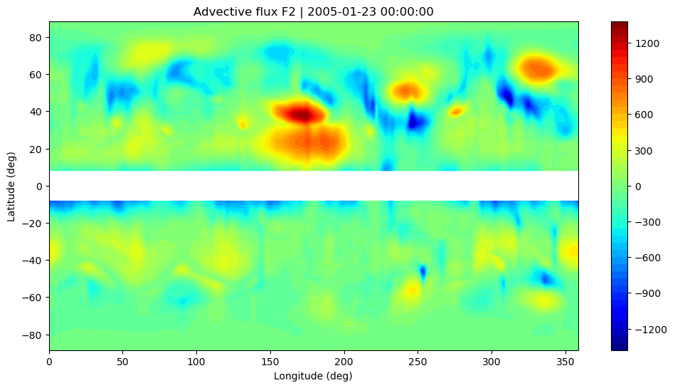
            (qgfield_object.adv_flux_f2, 'Advective flux F2'),
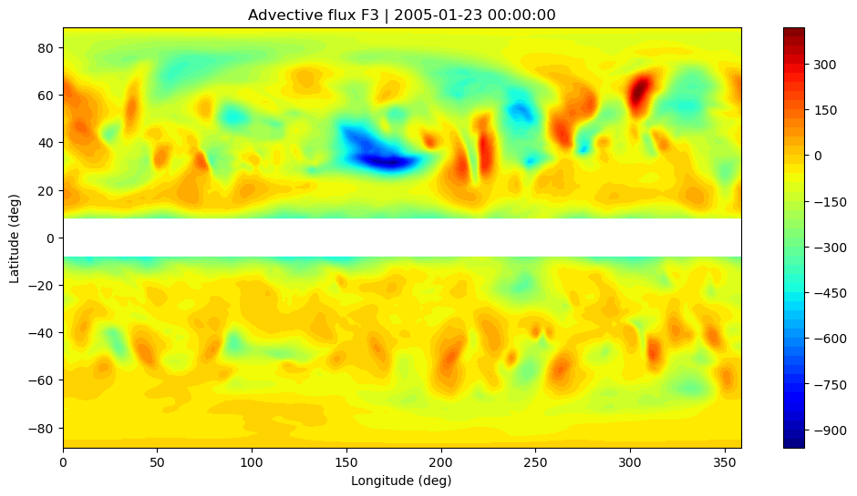
            (qgfield_object.adv_flux_f3, 'Advective flux F3'),
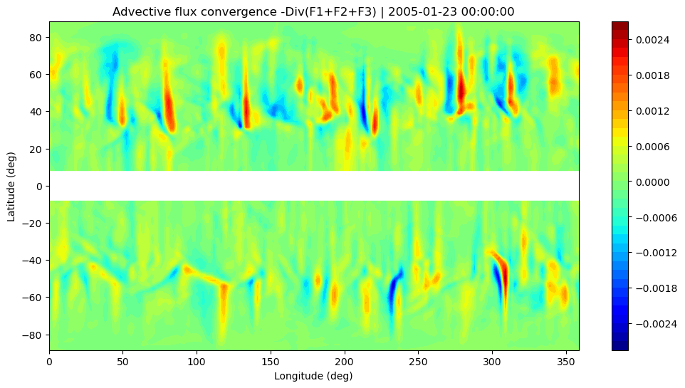
            (qgfield_object.convergence_zonal_advective_flux, 'Advective flux convergence -Div(F1+F2+F3)'),
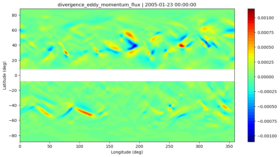
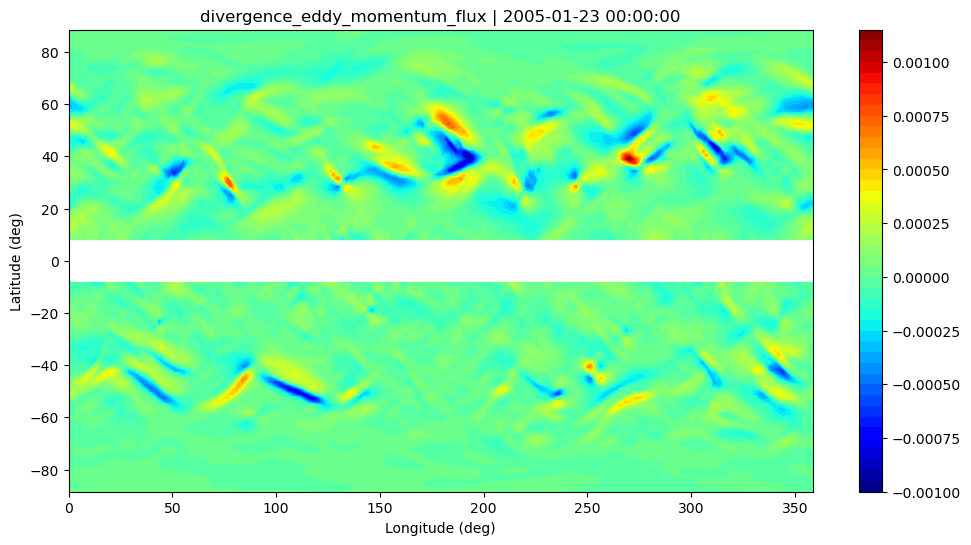
            (qgfield_object.divergence_eddy_momentum_flux, 'divergence_eddy_momentum_flux'),
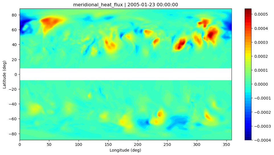
            (qgfield_object.meridional_heat_flux, 'meridional_heat_flux'),
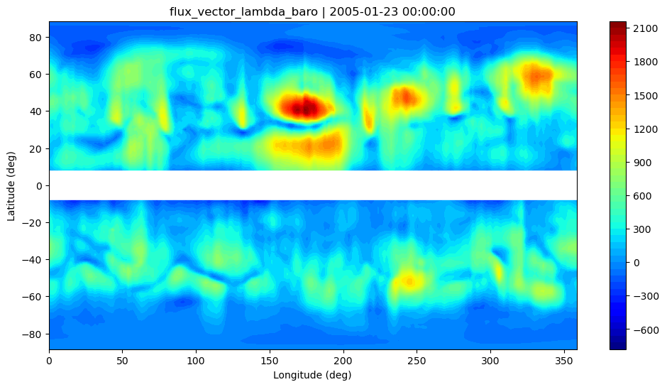
            (qgfield_object.flux_vector_lambda_baro, 'flux_vector_lambda_baro'),
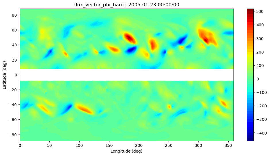
            (qgfield_object.flux_vector_phi_baro, 'flux_vector_phi_baro'),
        ]

        # Plot 240 hPa of 3D-variables
        for variable, name in variables_3d:
            plt.figure(figsize=(12,6))
            plt.contourf(xlon, ylat[1:-1], variable[plev_selected, 1:-1, :], 50, cmap='jet')
            if name=='Local wave activity (LWA)':
                plt.axhline(y=0, c='w', lw=30)
            plt.colorbar()
            plt.ylabel('Latitude (deg)')
            plt.xlabel('Longitude (deg)')
            plt.title(name + ' at 240hPa | ' + str(tstamp[tstep]))
            plt.show()

        # Plot reference states
        for variable, name in variables_yz:
            plt.figure(figsize=(6,4))
            plt.contourf(ylat[1:-1], height, variable[:, 1:-1], 50, cmap='jet')
            plt.axvline(x=0, c='w', lw=2)
            plt.xlabel('Latitude (deg)')
            plt.ylabel('Pseudoheight (m)')
            plt.colorbar()
            plt.title(name + ' | ' + str(tstamp[tstep]))
            plt.show()

        for variable, name in variables_xy:

            plt.figure(figsize=(12,6))
            plt.contourf(xlon, ylat[1:-1], variable[1:-1, :], 50, cmap='jet')
            plt.axhline(y=0, c='w', lw=30)
            plt.ylabel('Latitude (deg)')
            plt.xlabel('Longitude (deg)')
            plt.colorbar()
            plt.title(name + ' | ' + str(tstamp[tstep]))
            plt.show()


    print('tstep = {}/{}\n'.format(tstep, ntimes))

Do scipy interpolation
  1835044384           0           4  converged at n =          951
line 748: ncforce is None
  1835044384           0           4  converged at n =          727
 nd:           61 , jb:            0
 nd:           61 , jb:            0

tstep = 0/32

Do scipy interpolation
  1835044384           0           4  converged at n =          950
  1835044384           0           4  converged at n =          721
line 748: ncforce is None
 nd:           61 , jb:            0
 nd:           61 , jb:            0
tstep = 1/32

Do scipy interpolation
  1835044384           0           4  converged at n =          949
  1835044384           0           4  converged at n =          716
line 748: ncforce is None
 nd:           61 , jb:            0
 nd:           61 , jb:            0
tstep = 2/32

Do scipy interpolation
  1835044384           0           4  converged at n =          947
line 748: ncforce is None
  1835044384           0           4  converged at n =          719
 nd:           61 , jb:            0
 nd:           61 , jb:            0
tstep = 3/32

Do scipy interpolation
  1835044384           0           4  converged at n =          947
  1835044384           0           4  converged at n =          720
line 748: ncforce is None
 nd:           61 , jb:            0
 nd:           61 , jb:            0
tstep = 4/32

Do scipy interpolation
  1835044384           0           4  converged at n =          945
  1835044384           0           4  converged at n =          721
line 748: ncforce is None
 nd:           61 , jb:            0
 nd:           61 , jb:            0
tstep = 5/32

Do scipy interpolation
  1835044384           0           4  converged at n =          942
  1835044384           0           4  converged at n =          711
line 748: ncforce is None
 nd:           61 , jb:            0
 nd:           61 , jb:            0
tstep = 6/32

Do scipy interpolation
  1835044384           0           4  converged at n =          944
  1835044384           0           4  converged at n =          715
line 748: ncforce is None
 nd:           61 , jb:            0
 nd:           61 , jb:            0
tstep = 7/32

Do scipy interpolation
  1835044384           0           4  converged at n =          938
  1835044384           0           4  converged at n =          703
line 748: ncforce is None
 nd:           61 , jb:            0
 nd:           61 , jb:            0
tstep = 8/32

Do scipy interpolation
  1835044384           0           4  converged at n =          940
  1835044384           0           4  converged at n =          707
line 748: ncforce is None
 nd:           61 , jb:            0
 nd:           61 , jb:            0
tstep = 9/32

Do scipy interpolation
  1835044384           0           4  converged at n =          940
  1835044384           0           4  converged at n =          701
line 748: ncforce is None
 nd:           61 , jb:            0
 nd:           61 , jb:            0
tstep = 10/32

Do scipy interpolation
  1835044384           0           4  converged at n =          939
  1835044384           0           4  converged at n =          707
line 748: ncforce is None
 nd:           61 , jb:            0
 nd:           61 , jb:            0
tstep = 11/32

Do scipy interpolation
  1835044384           0           4  converged at n =          941
  1835044384           0           4  converged at n =          712
line 748: ncforce is None
 nd:           61 , jb:            0
 nd:           61 , jb:            0
tstep = 12/32

Do scipy interpolation
  1835044384           0           4  converged at n =          940
  1835044384           0           4  converged at n =          721
line 748: ncforce is None
 nd:           61 , jb:            0
 nd:           61 , jb:            0
tstep = 13/32

Do scipy interpolation
  1835044384           0           4  converged at n =          942
line 748: ncforce is None
  1835044384           0           4  converged at n =          718
 nd:           61 , jb:            0
 nd:           61 , jb:            0
tstep = 14/32

Do scipy interpolation
  1835044384           0           4  converged at n =          945
  1835044384           0           4  converged at n =          730
line 748: ncforce is None
 nd:           61 , jb:            0
 nd:           61 , jb:            0
tstep = 15/32

Do scipy interpolation
  1835044384           0           4  converged at n =          943
line 748: ncforce is None
  1835044384           0           4  converged at n =          731
 nd:           61 , jb:            0
 nd:           61 , jb:            0
tstep = 16/32

Do scipy interpolation
  1835044384           0           4  converged at n =          942
  1835044384           0           4  converged at n =          734
line 748: ncforce is None
 nd:           61 , jb:            0
 nd:           61 , jb:            0
tstep = 17/32

Do scipy interpolation
  1835044384           0           4  converged at n =          943
line 748: ncforce is None
  1835044384           0           4  converged at n =          734
 nd:           61 , jb:            0
 nd:           61 , jb:            0
tstep = 18/32

Do scipy interpolation
  1835044384           0           4  converged at n =          941
  1835044384           0           4  converged at n =          745
line 748: ncforce is None
 nd:           61 , jb:            0
 nd:           61 , jb:            0
tstep = 19/32

Do scipy interpolation
  1835044384           0           4  converged at n =          941
line 748: ncforce is None
  1835044384           0           4  converged at n =          744
 nd:           61 , jb:            0
 nd:           61 , jb:            0
tstep = 20/32

Do scipy interpolation
  1835044384           0           4  converged at n =          940
line 748: ncforce is None
  1835044384           0           4  converged at n =          746
 nd:           61 , jb:            0
 nd:           61 , jb:            0
tstep = 21/32

Do scipy interpolation
  1835044384           0           4  converged at n =          941
  1835044384           0           4  converged at n =          744
line 748: ncforce is None
 nd:           61 , jb:            0
 nd:           61 , jb:            0
tstep = 22/32

Do scipy interpolation
  1835044384           0           4  converged at n =          939
  1835044384           0           4  converged at n =          749
line 748: ncforce is None
 nd:           61 , jb:            0
 nd:           61 , jb:            0
tstep = 23/32

Do scipy interpolation
  1835044384           0           4  converged at n =          942
  1835044384           0           4  converged at n =          752
line 748: ncforce is None
 nd:           61 , jb:            0
 nd:           61 , jb:            0
tstep = 24/32

Do scipy interpolation
  1835044384           0           4  converged at n =          939
  1835044384           0           4  converged at n =          746
line 748: ncforce is None
 nd:           61 , jb:            0
 nd:           61 , jb:            0
tstep = 25/32

Do scipy interpolation
  1835044384           0           4  converged at n =          940
line 748: ncforce is None
  1835044384           0           4  converged at n =          734
 nd:           61 , jb:            0
 nd:           61 , jb:            0
tstep = 26/32

Do scipy interpolation
  1835044384           0           4  converged at n =          943
  1835044384           0           4  converged at n =          737
line 748: ncforce is None
 nd:           61 , jb:            0
 nd:           61 , jb:            0
tstep = 27/32

Do scipy interpolation
  1835044384           0           4  converged at n =          944
  1835044384           0           4  converged at n =          736
line 748: ncforce is None
 nd:           61 , jb:            0
 nd:           61 , jb:            0
tstep = 28/32

Do scipy interpolation
  1835044384           0           4  converged at n =          946
  1835044384           0           4  converged at n =          738
line 748: ncforce is None
 nd:           61 , jb:            0
 nd:           61 , jb:            0
tstep = 29/32

Do scipy interpolation
  1835044384           0           4  converged at n =          946
  1835044384           0           4  converged at n =          738
line 748: ncforce is None
 nd:           61 , jb:            0
 nd:           61 , jb:            0
tstep = 30/32

Do scipy interpolation
  1835044384           0           4  converged at n =          944
line 748: ncforce is None
  1835044384           0           4  converged at n =          740
 nd:           61 , jb:            0
 nd:           61 , jb:            0
tstep = 31/32