Object Oriented Interface

class oopinterface.QGField(xlon, ylat, plev, u_field, v_field, t_field, kmax=49, maxit=100000, dz=1000.0, npart=None, tol=1e-05, rjac=0.95, scale_height=falwa.constant.SCALE_HEIGHT, cp=falwa.constant.CP, dry_gas_constant=falwa.constant.DRY_GAS_CONSTANT, omega=falwa.constant.EARTH_OMEGA, planet_radius=falwa.constant.EARTH_RADIUS, northern_hemisphere_results_only=False, data_on_evenly_spaced_pseudoheight_grid=False, raise_error_for_nonconvergence=True)[source]: This class is equivalent to QGFieldNH18 for backward compatibility. QGField will be deprecated in upcoming release. See documentation in QGFieldNH18.

class oopinterface.QGFieldBase(xlon, ylat, plev, u_field, v_field, t_field, kmax=49, maxit=100000, dz=1000.0, npart=None, tol=1e-05, rjac=0.95, scale_height=falwa.constant.SCALE_HEIGHT, cp=falwa.constant.CP, dry_gas_constant=falwa.constant.DRY_GAS_CONSTANT, omega=falwa.constant.EARTH_OMEGA, planet_radius=falwa.constant.EARTH_RADIUS, northern_hemisphere_results_only=False, data_on_evenly_spaced_pseudoheight_grid=False, raise_error_for_nonconvergence=True)[source]

Local wave activity and flux analysis in the quasi-geostrophic framework.

Warning

This is an abstract class that defines the public interface but does not define any boundary conditions for the reference state computation. Instanciate via the specific child classes QGFieldNH18 or QGFieldNHN22 to select the desired boundary conditions.

Topography is assumed flat in this object.

New in version 0.3.0.

Parameters

xlon (numpy.array) – Array of evenly-spaced longitude (in degree) of size nlon.
ylat (numpy.array) – Array of evenly-spaced latitude (in degree) of size nlat. If it is a masked array, the value ylat.data will be used.
plev (numpy.) – Array of pressure level (in hPa) of size nlev.
u_field (numpy.ndarray) – Three-dimensional array of zonal wind field (in m/s) of dimension [nlev, nlat, nlon]. If it is a masked array, the value u_field.data will be used.
v_field (numpy.ndarray) – Three-dimensional array of meridional wind field (in m/s) of dimension [nlev, nlat, nlon]. If it is a masked array, the value v_field.data will be used.
t_field (numpy.ndarray) – Three-dimensional array of temperature field (in K) of dimension [nlev, nlat, nlon]. If it is a masked array, the value t_field.data will be used.
kmax (int, optional) – Dimension of uniform pseudoheight grids used for interpolation.
maxit (int, optional) – Number of iteration by the Successive over-relaxation (SOR) solver to compute the reference states.
dz (float, optional) – Size of uniform pseudoheight grids (in meters).
npart (int, optional) – Number of partitions used to compute equivalent latitude. If not initialized, it will be set to nlat.
tol (float, optional) – Tolerance that defines the convergence of solution in SOR solver.
rjac (float, optional) – Spectral radius of the Jacobi iteration in the SOR solver.
scale_height (float, optional) – Scale height of the atmosphere in meters. Default = 7000.
cp (float, optional) – Heat capacity of dry air in J/kg-K. Default = 1004.
dry_gas_constant (float, optional) – Gas constant for dry air in J/kg-K. Default = 287.
omega (float, optional) – Rotation rate of the earth in 1/s. Default = 7.29e-5.
planet_radius (float, optional) – Radius of the planet in meters. Default = 6.378e+6 (Earth’s radius).
northern_hemisphere_results_only (bool, optional) – whether only to return northern hemispheric results. Default = False
data_on_evenly_spaced_pseudoheight_grid (bool, optional) – whether the input data sits on an evenly spaced pseudoheight grid. Default = False If Ture, the method interpolate_fields (i.e. vertical interpolation) would not do vertical interpolation, but only calculate potential temperature, QGPV and static stability. New in version 1.3.
raise_error_for_nonconvergence (bool, optional) – If Uref solver does not have a solution, with this set to False, user can call compute_lwa_only after calling computer_reference_states. If set to True, an error is raised and the computation would halt.

property adv_flux_f1: Two-dimensional array of the second-order eddy term in zonal advective flux, i.e. F1 in equation 3 of NH18

property adv_flux_f2: Two-dimensional array of the third-order eddy term in zonal advective flux, i.e. F2 in equation 3 of NH18

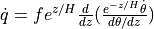
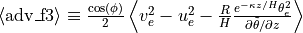
property adv_flux_f3: Two-dimensional array of the remaining term in zonal advective flux, i.e. F3 in equation 3 of NH18

abstract compute_layerwise_lwa_fluxes(ncforce=None)[source]: Compute layerwise lwa flux in Fortran except the stretching term, which will be calculated in python. Shall be in parallel with compute_lwa_and_barotropic_fluxes.

compute_lwa_and_barotropic_fluxes(return_named_tuple: bool = True, northern_hemisphere_results_only=None, ncforce=None)[source]

Compute barotropic components of local wave activity and flux terms in eqs.(2) and (3) in Nakamura and Huang (Science, 2018). It returns a named tuple called “LWA_and_fluxes” that consists of 9 elements as listed below. The discretization scheme that is used in the numerical integration is outlined in the Supplementary materials of Huang and Nakamura (GRL, 2017).

The parameter northern_hemisphere_results_only is deprecated and has no effect.

Note that flux computation for NHN22 is still experimental.

Parameters

return_named_tuple (bool) – Whether to returned a named tuple with variables in python indexing. Default: True. If False, nothing will be returned from this method. The variables can be retrieved from the QGField object after all computation is finished. This may save run time in some use case.
ncforce (optional, np.ndarray) – This is the diabatic term output from climate model interpolated on even-pseudoheight grid, i.e., the integrand of equation (12) in Lubis et al (2025, Nature Comm). The integrated barotropic component of ncforce is accessible via QGField.ncforce_baro.

Returns

adv_flux_f1 (numpy.ndarray) – Two-dimensional array of the second-order eddy term in zonal advective flux, i.e. F1 in equation 3 of NH18, with dimension = [nlat//2+1, nlon] if northern_hemisphere_results_only=True, or dimension = [nlat, nlon] if northern_hemisphere_results_only=False.
adv_flux_f2 (numpy.ndarray) – Two-dimensional array of the third-order eddy term in zonal advective flux, i.e. F2 in equation 3 of NH18, with dimension = [nlat//2+1, nlon] if northern_hemisphere_results_only=True, or dimension = [nlat, nlon] if northern_hemisphere_results_only=False.
adv_flux_f3 (numpy.ndarray) – Two-dimensional array of the remaining term in zonal advective flux, i.e. F3 in equation 3 of NH18, with dimension = [nlat//2+1, nlon] if northern_hemisphere_results_only=True, or dimension = [nlat, nlon] if northern_hemisphere_results_only=False.
convergence_zonal_advective_flux (numpy.ndarray) – Two-dimensional array of the convergence of zonal advective flux, i.e. -div(F1+F2+F3) in equation 3 of NH18, with dimension = [nlat//2+1, nlon] if northern_hemisphere_results_only=True, or dimension = [nlat, nlon] if northern_hemisphere_results_only=False.
divergence_eddy_momentum_flux (numpy.ndarray) – Two-dimensional array of the divergence of eddy momentum flux, i.e. (II) in equation 2 of NH18, with dimension = [nlat//2+1, nlon] if northern_hemisphere_results_only=True, or dimension = [nlat, nlon] if northern_hemisphere_results_only=False.
meridional_heat_flux (numpy.ndarray) – Two-dimensional array of the low-level meridional heat flux, i.e. (III) in equation 2 of NH18, with dimension = [nlat//2+1, nlon] if northern_hemisphere_results_only=True, or dimension = [nlat, nlon] if northern_hemisphere_results_only=False.
lwa_baro (np.ndarray) – Two-dimensional array of barotropic local wave activity (with cosine weighting). Dimension = [nlat//2+1, nlon] if northern_hemisphere_results_only=True, or dimension = [nlat, nlon] if northern_hemisphere_results_only=False.
u_baro (np.ndarray) – Two-dimensional array of barotropic zonal wind (without cosine weighting). Dimension = [nlat//2+1, nlon] if northern_hemisphere_results_only=True, or dimension = [nlat, nlon] if northern_hemisphere_results_only=False.
lwa (np.ndarray) – Three-dimensional array of barotropic local wave activity Dimension = [kmax, nlat//2+1, nlon] if northern_hemisphere_results_only=True, or dimension = [kmax, nlat, nlon] if northern_hemisphere_results_only=False.

Examples

>>> adv_flux_f1, adv_flux_f2, adv_flux_f3, convergence_zonal_advective_flux,
    divergence_eddy_momentum_flux, meridional_heat_flux,
    lwa_baro, u_baro, lwa = test_object.compute_lwa_and_barotropic_fluxes()

compute_lwa_only() → None[source]

New in version 1.3. After calling compute_reference_state, if the reference state Uref was not solved properly, this method would compute LWA (and its barotropic component) based on QGPV and Qref obtained from previous step.

Note with caution that, the implementation of this method in QGFieldNH18 behaves slightly differently from compute_lwa_and_barotropic_fluxes in the Southern Hemisphere (while it produces the same results for the Northern Hemisphere) probably due to indexing difference.

To retrieve LWA and barotropic fluxes computed:

>>> QGField.compute_lwa_only()
>>> lwa_baro = QGField.lwa_baro  # barotropic LWA
>>> u_baro = QGField.u_baro    # barotropic U
>>> lwa = QGField.lwa       # 3-D LWA

compute_ncforce_from_heating_rate(heating_rate)[source]

Parameters

heating_rate (np.array) – The diabatic heating rate, i.e. tendency of potential temperature, $\dot{ \theta } \equiv \frac{ d \theta }{dt}$ at pressure levels that has unit K/s.
stat_n (np.array) – 1-d numpy array of northern-hemispheric averaged static stability
stat_s (np.array) – 1-d numpy array of southern-hemispheric averaged static stability

Returns

Array that contains the ncforce term $\dot{ q } = f e^{z/H} \frac{d}{dz} ( \frac{e^{-z/H} \dot{\theta}}{d\theta/dz})$

Return type

np.ndarray

compute_reference_states(return_named_tuple: bool = True, northern_hemisphere_results_only=None) → Optional[NamedTuple][source]

Compute the local wave activity and reference states of QGPV, zonal wind and potential temperature using a more stable inversion algorithm applied in Nakamura and Huang (2018, Science). The equation to be invert is equation (22) in supplementary materials of Huang and Nakamura (2017, GRL).

The parameter northern_hemisphere_results_only is deprecated and has no effect.

Parameters

return_named_tuple (bool) – Whether to returned a named tuple with variables in python indexing. Default: True. If False, nothing will be returned from this method. The variables can be retrieved from the QGField object after all computation is finished. This may save run time in some use case.

Returns

Qref (numpy.ndarray) – Two-dimensional array of reference state of quasi-geostrophic potential vorticity (QGPV) with dimension = [kmax, nlat, nlon] if northern_hemisphere_results_only=False, or dimension = [kmax, nlat//2+1, nlon] if northern_hemisphere_results_only=True
Uref (numpy.ndarray) – Two-dimensional array of reference state of zonal wind (Uref) with dimension = [kmax, nlat, nlon] if northern_hemisphere_results_only=False, or dimension = [kmax, nlat//2+1, nlon] if northern_hemisphere_results_only=True
PTref (numpy.ndarray) – Two-dimensional array of reference state of potential temperature (Theta_ref) with dimension = [kmax, nlat, nlon] if northern_hemisphere_results_only=False, or dimension = [kmax, nlat//2+1, nlon] if northern_hemisphere_results_only=True

Examples

>>> qref, uref, ptref = test_object.compute_reference_states()

property convergence_zonal_advective_flux: Two-dimensional array of the convergence of zonal advective flux, i.e. -div(F1+F2+F3) in equation 3 of NH18

property divergence_eddy_momentum_flux: Two-dimensional array of the divergence of eddy momentum flux, i.e. (II) in equation 2 of NH18

property ep1: Layerwise meridional eddy momentum flux convergence (adv_flux_f3/layerwize F3 in NH18).

property ep2

np.ndarray of dimension(kmax, nlat, nlon):: the discretized meridional eddy momentum flux divergence at grid point j is computed by

$\frac{[\text{ep2} - \text{ep3}]}{a (2 \Delta\phi) \cos{\phi}}$ where $\text{ep2} \equiv (u_e v_e cos^2(\phi+\phi^\prime))_{j+1}$ and $\text{ep3} \equiv (u_e v_e cos^2(\phi+\phi^\prime))_{j-1}$

property ep3

np.ndarray of dimension(kmax, nlat, nlon):: the discretized meridional eddy momentum flux divergence at grid point j is computed by

$\frac{[\text{ep2} - \text{ep3}]}{a (2 \Delta\phi) \cos{\phi}}$ where $\text{ep2} \equiv (u_e v_e cos^2(\phi+\phi^\prime))_{j+1}$ and $\text{ep3} \equiv (u_e v_e cos^2(\phi+\phi^\prime))_{j-1}$

property flux_vector_lambda_baro

np.ndarray of dimension(nlat, nlon):: Barotropic zonal wave activity flux vector, i.e. eq. (6) of Lee and Nakamura (2024):

where $\langle F_\lambda \rangle = \langle \text{adv\_f1} \rangle + \langle \text{adv\_f2} \rangle + \langle \text{adv\_f3} \rangle$ , $\langle \text{adv\_f1} \rangle \equiv \langle u_\mathrm{REF} A \cos(\phi) \rangle$ , $\langle \text{adv\_f2} \rangle \equiv - a \langle \int_0^{\Delta\phi} u_e q_e \cos(\phi + \phi') \mathrm{d}\phi^\prime \rangle$ , $\langle \text{adv\_f3} \rangle \equiv \frac{\cos(\phi)}{2} \left\langle v_e^2 - u_e^2 - \frac{R}{H} \frac{e^{-\kappa z / H} \theta_e^2}{\partial \tilde\theta / \partial z} \right\rangle$

property flux_vector_phi_baro

np.ndarray of dimension(nlat, nlon):: Barotropic meridional wave activity flux vector, i.e. eq. (7) of Lee and Nakamura (2024):

$\langle F_\lambda \rangle = - \langle u_e * v_e \rangle * cos(\phi)$

Computed as -0.5 * (ep2baro + ep3baro) / cos(phi).

get_latitude_dim()[source]: Return the latitude dimension of the input data.

interpolate_fields(return_named_tuple: bool = True) → Optional[NamedTuple][source]

Interpolate zonal wind, maridional wind, and potential temperature field onto the uniform pseudoheight grids, and compute QGPV on the same grids. This returns named tuple called “Interpolated_fields” that consists of 5 elements as listed below.

Parameters

return_named_tuple (bool) – Whether to returned a named tuple with variables in python indexing. Default: True. If False, nothing will be returned from this method. The variables can be retrieved from the QGField object after all computation is finished. This may save run time in some use case.

Returns

QGPV (numpy.ndarray) – Three-dimensional array of quasi-geostrophic potential vorticity (QGPV) with dimension = [kmax, nlat, nlon]
U (numpy.ndarray) – Three-dimensional array of interpolated zonal wind with dimension = [kmax, nlat, nlon]
V (numpy.ndarray) – Three-dimensional array of interpolated meridional wind with dimension = [kmax, nlat, nlon]
Theta (numpy.ndarray) – Three-dimensional array of interpolated potential temperature with dimension = [kmax, nlat, nlon]
Static_stability (numpy.array) – One-dimension array of interpolated static stability with dimension = kmax

Examples

>>> interpolated_fields = test_object.interpolate_fields()
>>> interpolated_fields.QGPV  # This is to access the QGPV field

property interpolated_theta: Potential temperature on the regular pseudoheight grids.

property interpolated_u: Zonal wind on the regular pseudoheight grids.

property interpolated_v: Meridional wind on the regular pseudoheight grids.

property layerwise_flux_terms_storage: falwa.data_storage.LayerwiseFluxTermsStorage

Return the LayerwiseFluxTermsStorage object that stored the following 3D LWA and flux terms on pseudo-height levels. The layerwise flux terms are only computed after calling the method QGField.compute_layerwise_lwa_fluxes.

Returns

lwa: Total local wave activity
astar1: cyclonic (for N. Hem.) local wave activity
astar2: anti-cyclonic (for N. Hem.) local wave activity
ua1: first/linear term of zonal advective flux
ua2: second/nonlinear term of zonal advective flux
ep1: third term (F3 in NH18) of zonal advective flux
ep2 and ep3: the discretized meridional eddy momentum flux divergence at grid point j is computed by

$\frac{[\text{ep2} - \text{ep3}]}{a (2 \Delta\phi) \cos{\phi}}$ where $\text{ep2} \equiv (u_e v_e cos^2(\phi+\phi^\prime))_{j+1}$ and $\text{ep3} \equiv (u_e v_e cos^2(\phi+\phi^\prime))_{j-1}$

stretch_term: layerwise stretch term corresponding to III in NH18 eq (2)
ncforce: layerwise contribution of input heating term

Return type

A LayerwiseFluxTermsStorage object that contains the following 3D fields of LWA and flux terms (without density weighting)

property lwa: Three-dimensional array of local wave activity

property lwa_baro: Two-dimensional array of barotropic local wave activity (with cosine weighting).

property meridional_heat_flux: Two-dimensional array of the low-level meridional heat flux, i.e. (III) in equation 2 of NH18

property ncforce_baro: If input ncforce of method compute_lwa_and_barotropic_fluxes is not None, this would return the corresponding barotropic component of non-conservative force contribution with respect to the wave activity budget equation in Lubis et al (2025, Nature Comm) Eq.(11).

property nonconvergent_uref: bool

If True, QGField.compute_lwa_and_barotropic_flux cannot be called. If user deems appropriate to proceed with LWA calculation, call QGField.compute_lwa_only instead.

Return type: A boolean. Initial value is False. After calling QGField.compute_reference_state, if Uref cannot be solved, its value will be changed to True.

property northern_hemisphere_results_only: bool: Even though a global field is required for input, whether ref state and fluxes are computed for northern hemisphere only

property prefactor: Normalization constant for vertical weighted-averaged integration

property ptref: Reference state of potential temperature (Theta_ref).

property qgpv: Quasi-geostrophic potential vorticity on the regular pseudoheight grids.

property qref: Reference state of QGPV (Qref).

abstract property static_stability: Union[array, Tuple[array, array]]: The interpolated static stability.

property stretch_term

np.ndarray of dimension(kmax, nlat, nlon): This is the stretch term that is present only in the layerwise LWA budget equation in Lubis et al (2025), but not the barotropic LWA budget equation in NH18/NHN22. The vertical average of this term is the low-level meridional heat flux. The expression of the stretch term is:

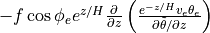
$- f\cos\phi_e e^{z/H}\frac{\partial}{\partial z}\left( \frac{ e^{-z/H} v_e \theta_e}{\partial\tilde\theta/\partial z} \right)$

It is only computed after calling QGField.compute_layerwise_lwa_fluxes.

property u_baro: Two-dimensional array of barotropic zonal wind (without cosine weighting).

property ua1: Layerwise first/linear term of zonal advective flux (adv_flux_f1/layerwize F1 in NH18).

property ua2: Layerwise second/nonlinear term of zonal advective flux (adv_flux_f2/layerwize F2 in NH18).

property uref: Reference state of zonal wind (Uref).

property ylat: This is ylat grid input by user.

property ylat_ref_states: array: This is the reference state grid output to user

property ylat_ref_states_analysis: array: Latitude dimension of reference state. This is input to ReferenceStatesStorage.qref_correct_unit.

class oopinterface.QGFieldNH18(xlon, ylat, plev, u_field, v_field, t_field, kmax=49, maxit=100000, dz=1000.0, npart=None, tol=1e-05, rjac=0.95, scale_height=falwa.constant.SCALE_HEIGHT, cp=falwa.constant.CP, dry_gas_constant=falwa.constant.DRY_GAS_CONSTANT, omega=falwa.constant.EARTH_OMEGA, planet_radius=falwa.constant.EARTH_RADIUS, northern_hemisphere_results_only=False, data_on_evenly_spaced_pseudoheight_grid=False, raise_error_for_nonconvergence=True)[source]

Procedures and reference state computation with the set of boundary conditions of NH18:

Nakamura, N., & Huang, C. S. (2018). Atmospheric blocking as a traffic jam in the jet stream. Science, 361(6397), 42-47. https://www.science.org/doi/10.1126/science.aat0721

See the documentation of QGField for the public interface. There are no additional arguments for this class.

New in version 0.7.0.

Examples

Demo script for the analyses done in Nakamura and Huang (2018, Science)

compute_layerwise_lwa_fluxes(ncforce=None)[source]: Compute layerwise lwa flux in Fortran except the stretching term, which will be calculated in python. Shall be in parallel with compute_lwa_and_barotropic_fluxes.

property static_stability: array: The interpolated static stability.

class oopinterface.QGFieldNHN22(xlon, ylat, plev, u_field, v_field, t_field, kmax=49, maxit=100000, dz=1000.0, npart=None, tol=1e-05, rjac=0.95, scale_height=falwa.constant.SCALE_HEIGHT, cp=falwa.constant.CP, dry_gas_constant=falwa.constant.DRY_GAS_CONSTANT, omega=falwa.constant.EARTH_OMEGA, planet_radius=falwa.constant.EARTH_RADIUS, northern_hemisphere_results_only=False, eq_boundary_index=5, data_on_evenly_spaced_pseudoheight_grid=False)[source]

Procedures and reference state computation with the set of boundary conditions of NHN22:

Neal et al (2022). The 2021 Pacific Northwest heat wave and associated blocking: meteorology and the role of an upstream cyclone as a diabatic source of wave activity. https://agupubs.onlinelibrary.wiley.com/doi/full/10.1029/2021GL097699

Note that barotropic flux term computation from this class occasionally experience numerical instability, so please use with caution.

See the documentation of QGField for the public interface.

New in version 0.7.0.

Parameters: eq_boundary_index (int, optional) – The improved inversion algorithm of reference states allow modification of equatorward boundary to be the absolute vorticity. This parameter specify the location of grid point (from equator) which will be used as boundary. The results in NHN22 is produced by using 1 deg latitude data and eq_boundary_index = 5, i.e. using a latitude domain from 5 deg to the pole. Default = 5 here.

Examples

Notebook: Direct inversion algorithm for reference state computation (Neal et al 2023 GRL)

compute_layerwise_lwa_fluxes(ncforce=None)[source]: Compute layerwise lwa flux in Fortran except the stretching term, which will be calculated in python. Shall be in parallel with compute_lwa_and_barotropic_fluxes.

property static_stability: Tuple[array, array]: The interpolated static stability.

Terms in the LWA Column Budget

There are two sets of methods to compute the LWA column budget available:

Nakamura and Huang, Science (2018)QGFieldNH18.
Eq (2), (3) with reference states solved with boundary conditions (S4) and SOR.
Neal et al., GRL (2022)QGFieldNHN22.
Eq (S5) - (S7) with reference states solved with boundary conditions (S14) - (S16) and direct inversion (since the latitudinal boundary is away from the equator, solution is guaranteed).

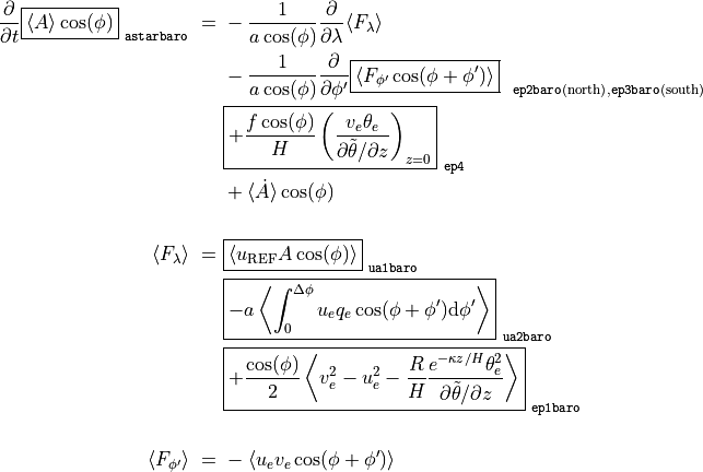
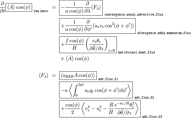
With the LWA column budget as formulated by Nakamura and Huang, Science (2018), the output fields of QGField.compute_lwa_and_barotropic_fluxes() correspond to terms as follows:

$\frac{\partial}{\partial t} \boxed{ \langle A \rangle \cos(\phi) }_\mathtt{~lwa\_baro} ~ = ~ & \boxed{ - \frac{1}{a \cos(\phi)} \frac{\partial}{\partial \lambda} \langle F_{\lambda} \rangle }_\mathtt{~convergence\_zonal\_advective\_flux} \\ & \boxed{ + \frac{1}{a \cos(\phi)} \frac{\partial}{\partial \phi'} \langle u_e v_e \cos^2(\phi + \phi') \rangle }_\mathtt{~divergence\_eddy\_momentum\_flux} \\ & \boxed{ + \frac{f \cos(\phi)}{H} \left( \frac{v_e \theta_e}{\partial \tilde\theta / \partial z} \right)_{z=0} }_\mathtt{~meridional\_heat\_flux} \\ & + \langle \dot A \rangle \cos(\phi) \\ \langle F_{\lambda} \rangle ~ = ~ & \boxed{ \langle u_\mathrm{REF} A \cos(\phi) \rangle }_\mathtt{~adv\_flux\_f1} \\ & \boxed{ - a \left\langle \int_0^{\Delta\phi} u_e q_e \cos(\phi + \phi') \mathrm{d}\phi' \right\rangle }_\mathtt{~adv\_flux\_f2} \\ & \boxed{ + \frac{\cos(\phi)}{2} \left\langle v_e^2 - u_e^2 - \frac{R}{H} \frac{e^{-\kappa z / H} \theta_e^2}{\partial \tilde\theta / \partial z} \right\rangle }_\mathtt{~adv\_flux\_f3} \\$

Note

Before version 0.7.0, the routines used in Neal et al., GRL (2022) were encapsulated in implicit functions:

_interpolate_field_dirinv

_compute_qref_fawa_and_bc

_compute_lwa_flux_dirinv

With output fields of _compute_lwa_flux_dirinv corresponding to the terms of the LWA budget in the following way:

$\frac{\partial}{\partial t} \boxed{ \langle A \rangle \cos(\phi) }_\mathtt{~astarbaro} ~ = ~ & - \frac{1}{a \cos(\phi)} \frac{\partial}{\partial \lambda} \langle F_{\lambda} \rangle \\ & - \frac{1}{a \cos(\phi)} \frac{\partial}{\partial \phi'} \boxed{ \langle F_{\phi'} \cos(\phi + \phi') \rangle }_{~\mathtt{~ep2baro} \mathrm{(north)}, \mathtt{ep3baro} \mathrm{(south)}} \\ & \boxed{ + \frac{f \cos(\phi)}{H} \left( \frac{v_e \theta_e}{\partial \tilde\theta / \partial z} \right)_{z=0} }_\mathtt{~ep4} \\ & + \langle \dot A \rangle \cos(\phi) \\ \langle F_{\lambda} \rangle ~ = ~ & \boxed{ \langle u_\mathrm{REF} A \cos(\phi) \rangle }_\mathtt{~ua1baro} \\ & \boxed{ - a \left\langle \int_0^{\Delta\phi} u_e q_e \cos(\phi + \phi') \mathrm{d}\phi' \right\rangle }_\mathtt{~ua2baro} \\ & \boxed{ + \frac{\cos(\phi)}{2} \left\langle v_e^2 - u_e^2 - \frac{R}{H} \frac{e^{-\kappa z / H} \theta_e^2}{\partial \tilde\theta / \partial z} \right\rangle }_\mathtt{~ep1baro} \\ \langle F_{\phi'} \rangle ~ = ~ & - \langle u_e v_e \cos(\phi + \phi') \rangle$