Last updated on Nov 5, 2023

Direct inversion algorithm for reference state computation (Neal et al 2023 GRL)

This notebook computes LWA and reference states from the same dataset as in demo_script_for_nh2018.ipynb but use the new boundary conditions outlined in NHN22:

Neal, E., Huang, C. S., & Nakamura, N. (2022). The 2021 Pacific Northwest heat wave and associated blocking: meteorology and the role of an upstream cyclone as a diabatic source of wave activity. Geophysical Research Letters, 49(8), e2021GL097699.

See the code under Additional parameters needed to switch to NHN22 boundary conditions for additional parameters needed to compute reference states with NHN22 boundary conditions.

From release v0.7.0, users can choose the version of boundary conditions to compute reference states via the child class of QGField. To compute reference states using boundary condition in NHN22 with a dataset of $1^\circ\times1^\circ$ grid resolution, one could initialized the corresponding QGField child class:

QGFieldNHN22(xlon, ylat, plev, uu, vv, tt, eq_boundary_index=5)

which corresponds to an equatorward boundary at $5^\circ$ N.

This notebook is using a dataset of $1.5^\circ\times1.5^\circ$ grid resolution such that eq_boundary_index=3 refers to an equatorward boundary at $4.5^\circ$ N.

Please raise an issue in the GitHub repo or contact Clare S. Y. Huang (csyhuang@uchicago.edu) if you have any questions or suggestions regarding the package.

[1]:

import numpy as np
import xarray as xr
from numpy import dtype
from math import pi
from netCDF4 import Dataset
import matplotlib.pyplot as plt
import datetime as dt
%matplotlib inline
from falwa.oopinterface import QGFieldNHN22
import falwa.utilities as utilities
import datetime as dt

Load the dimension arrays

In this version, the QGField object takes only: - latitude array in degree ascending order, and - pressure level in hPa in decending order (from ground to aloft).

[4]:

xlon = u_file.longitude.values

# latitude has to be in ascending order
ylat = u_file.latitude.values
if np.diff(ylat)[0]<0:
    print('Flip ylat.')
    ylat = ylat[::-1]

# pressure level has to be in descending order (ascending height)
plev = u_file.level.values
if np.diff(plev)[0]>0:
    print('Flip plev.')
    plev = plev[::-1]

nlon = xlon.size
nlat = ylat.size
nlev = plev.size

Flip ylat.
Flip plev.

[5]:

clat = np.cos(np.deg2rad(ylat))     # cosine latitude
p0 = 1000.                          # surface pressure [hPa]
kmax = 49                           # number of grid points for vertical extrapolation (dimension of height)
dz = 1000.                          # differential height element
height = np.arange(0,kmax)*dz       # pseudoheight [m]
dphi = np.diff(ylat)[0]*pi/180.     # differential latitudinal element
dlambda = np.diff(xlon)[0]*pi/180.  # differential latitudinal element
hh = 7000.                          # scale height
cp = 1004.                          # heat capacity of dry air
rr = 287.                           # gas constant
omega = 7.29e-5                     # rotation rate of the earth
aa = 6.378e+6                       # earth radius
prefactor = np.array([np.exp(-z/hh) for z in height[1:]]).sum() # integrated sum of density from the level
                                                                #just above the ground (z=1km) to aloft
npart = nlat                        # number of partitions to construct the equivalent latitude grids
maxits = 100000                     # maximum number of iteration in the SOR solver to solve for reference state
tol = 1.e-5                         # tolerance that define convergence of solution
rjac = 0.95                         # spectral radius of the Jacobi iteration in the SOR solver.
jd = nlat//2+1                      # (one plus) index of latitude grid point with value 0 deg
                                    # This is to be input to fortran code. The index convention is different.

Set the level of pressure and the timestamp to display below

[6]:

tstamp = [dt.datetime(2005,1,23,0,0) + dt.timedelta(seconds=6*3600) * tt for tt in range(ntimes)]
plev_selected = 10 # selected pressure level to display
tstep_selected = 0

Additional parameters to compute reference state from NHN22 boundary conditions

This dataset has $1.5^\circ$ latitude resolution. eq_boundary_index = 3 refers to an equatorward boundary at $4.5^\circ$ N

[7]:

eq_boundary_index = 3

Loop through the input file and store all the computed quantities in a netCDF file

[8]:

for tstep in range(32):  # or ntimes

    uu = u_file.variables['u'][tstep, ::-1, ::-1, :].data
    vv = v_file.variables['v'][tstep, ::-1, ::-1, :].data
    tt = t_file.variables['t'][tstep, ::-1, ::-1, :].data

    qgfield_object = QGFieldNHN22(
        xlon, ylat, plev, uu, vv, tt, eq_boundary_index=eq_boundary_index, northern_hemisphere_results_only=False)
    equator_idx = qgfield_object.equator_idx

    qgfield_object.interpolate_fields(return_named_tuple=False)

    qgfield_object.compute_reference_states(return_named_tuple=False)

    qgfield_object.compute_lwa_and_barotropic_fluxes(return_named_tuple=False)

    if tstep == tstep_selected:
        # === Below demonstrate another way to access the computed variables ===
        # 3D Variables that I would choose one pressure level to display
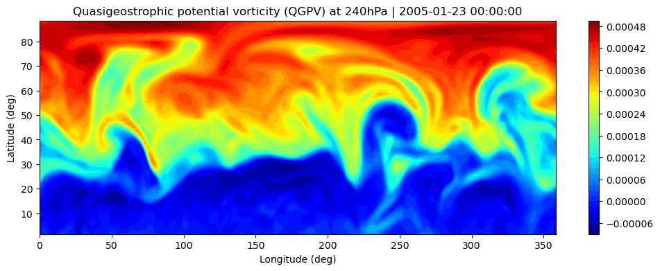
        variables_3d = [
            (qgfield_object.qgpv, 'Quasigeostrophic potential vorticity (QGPV)'),
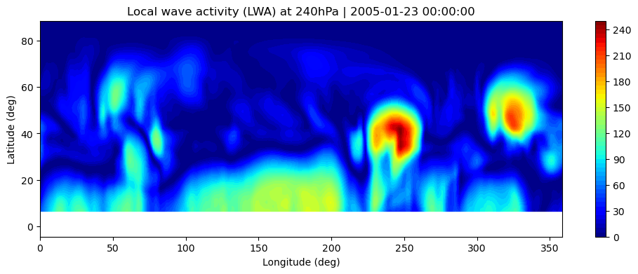
            (qgfield_object.lwa, 'Local wave activity (LWA)'),
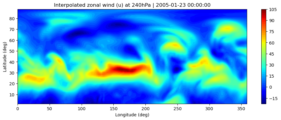
            (qgfield_object.interpolated_u, 'Interpolated zonal wind (u)'),
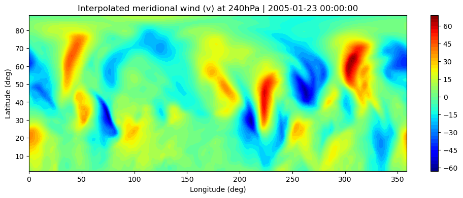
            (qgfield_object.interpolated_v, 'Interpolated meridional wind (v)')]

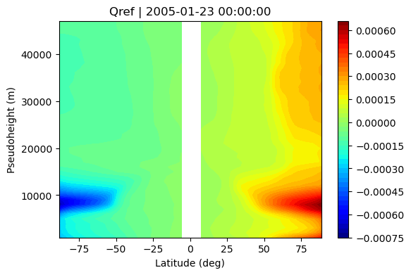
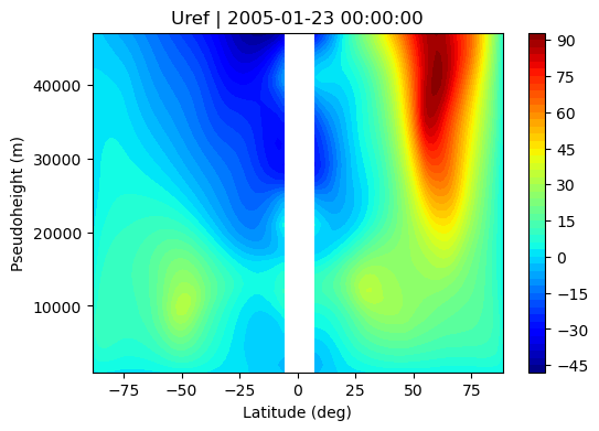
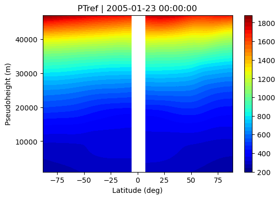
        # Reference states to be displayed on y-z plane
        variables_yz = [
            (qgfield_object.qref, 'Qref'),
            (qgfield_object.uref, 'Uref'),
            (qgfield_object.ptref, 'PTref')]

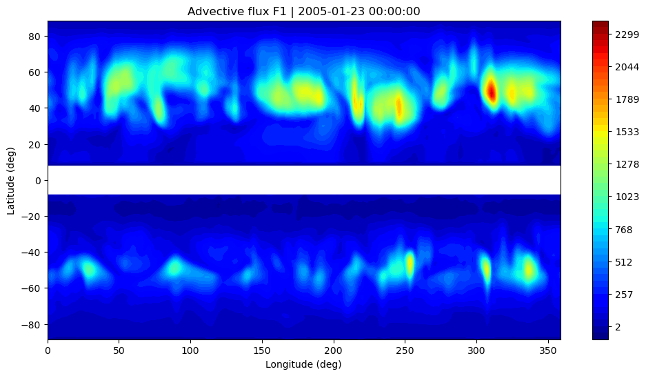
        # Vertically averaged variables to be displayed on x-y plane
        variables_xy = [
            (qgfield_object.adv_flux_f1, 'Advective flux F1'),
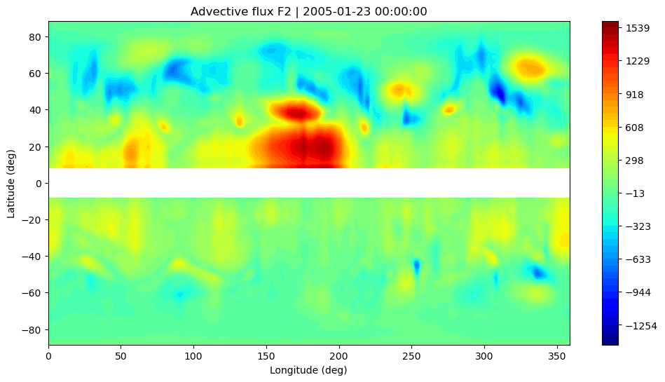
            (qgfield_object.adv_flux_f2, 'Advective flux F2'),
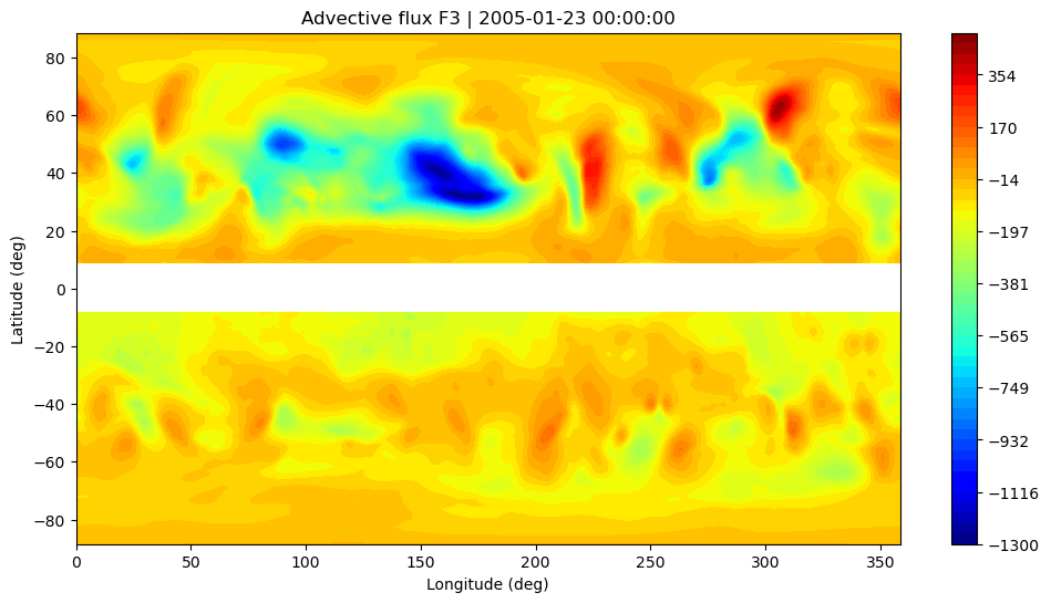
            (qgfield_object.adv_flux_f3, 'Advective flux F3'),
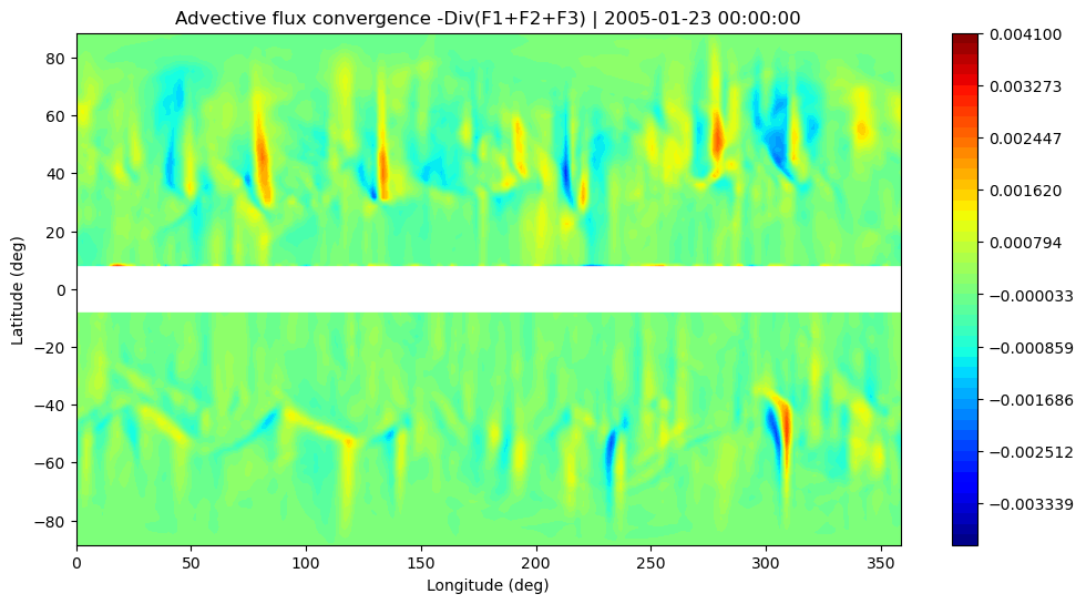
            (qgfield_object.convergence_zonal_advective_flux, 'Advective flux convergence -Div(F1+F2+F3)'),
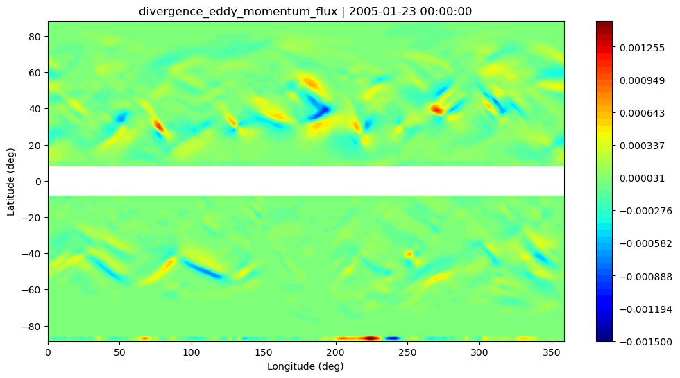
            (qgfield_object.divergence_eddy_momentum_flux, 'divergence_eddy_momentum_flux'),
            (qgfield_object.meridional_heat_flux, 'meridional_heat_flux')
        ]

        # Plot 240 hPa of 3D-variables
        for variable, name in variables_3d:
            plt.figure(figsize=(12,4))
            plt.contourf(xlon, ylat[equator_idx:-1], variable[plev_selected, equator_idx:-1, :], 50, cmap='jet')
            if name=='Local wave activity (LWA)':
                plt.axhline(y=0, c='w', lw=30)
            plt.colorbar()
            plt.ylabel('Latitude (deg)')
            plt.xlabel('Longitude (deg)')
            plt.title(name + ' at 240hPa | ' + str(tstamp[tstep]))
            plt.show()

        # Plot reference states
        for variable, name in variables_yz:
            # Mask out equatorward region that is outside analysis boundary
            mask = np.zeros_like(variable)
            mask[:, equator_idx-eq_boundary_index-1:equator_idx+eq_boundary_index+1] = np.nan
            variable_masked = np.ma.array(variable, mask=mask)
            # Start plotting
            plt.figure(figsize=(6,4))
            plt.contourf(ylat[1:-1], height[1:-1], variable_masked[1:-1, 1:-1], 50, cmap='jet')
            plt.axvline(x=0, c='w', lw=2)
            plt.xlabel('Latitude (deg)')
            plt.ylabel('Pseudoheight (m)')
            plt.colorbar()
            plt.title(name + ' | ' + str(tstamp[tstep]))
            plt.show()

        # Plot fluxes (color axies have to be fixed)
        plt.figure(figsize=(12,6))
        plt.contourf(xlon, ylat[1:-1], variables_xy[0][0][1:-1, :], np.linspace(-100, 2401, 50), cmap='jet')
        plt.axhline(y=0, c='w', lw=30)
        plt.ylabel('Latitude (deg)')
        plt.xlabel('Longitude (deg)')
        plt.colorbar()
        plt.title(variables_xy[0][1] + ' | ' + str(tstamp[tstep]))
        plt.show()

        plt.figure(figsize=(12,6))
        plt.contourf(xlon, ylat[1:-1], variables_xy[1][0][1:-1, :], np.linspace(-1440, 1601, 50), cmap='jet')
        plt.axhline(y=0, c='w', lw=30)
        plt.ylabel('Latitude (deg)')
        plt.xlabel('Longitude (deg)')
        plt.colorbar()
        plt.title(variables_xy[1][1] + ' | ' + str(tstamp[tstep]))
        plt.show()

        plt.figure(figsize=(12,6))
        plt.contourf(xlon, ylat[1:-1], variables_xy[2][0][1:-1, :], np.linspace(-1300, 501, 50), cmap='jet')
        plt.axhline(y=0, c='w', lw=30)
        plt.ylabel('Latitude (deg)')
        plt.xlabel('Longitude (deg)')
        plt.colorbar()
        plt.title(variables_xy[2][1] + ' | ' + str(tstamp[tstep]))
        plt.show()

        plt.figure(figsize=(12,6))
        plt.contourf(xlon, ylat[1:-1], variables_xy[3][0][1:-1, :], np.linspace(-0.004, 0.0041, 50), cmap='jet')
        plt.axhline(y=0, c='w', lw=30)
        plt.ylabel('Latitude (deg)')
        plt.xlabel('Longitude (deg)')
        plt.colorbar()
        plt.title(variables_xy[3][1] +' | ' + str(tstamp[tstep]))
        plt.show()

        plt.figure(figsize=(12,6))
        plt.contourf(xlon, ylat[1:-1], variables_xy[4][0][1:-1, :], np.linspace(-0.0015, 0.0015, 50), cmap='jet')
        plt.axhline(y=0, c='w', lw=30)
        plt.ylabel('Latitude (deg)')
        plt.xlabel('Longitude (deg)')
        plt.colorbar()
        plt.title(variables_xy[4][1] +' | ' + str(tstamp[tstep]))
        plt.show()

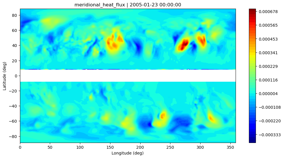
        plt.figure(figsize=(12,6))
        plt.contourf(xlon, ylat[1:-1], variables_xy[5][0][1:-1, :], np.linspace(-0.0004, 0.0007, 50), cmap='jet')
        plt.axhline(y=0, c='w', lw=30)
        plt.ylabel('Latitude (deg)')
        plt.xlabel('Longitude (deg)')
        plt.colorbar()
        plt.title(variables_xy[5][1] +' | ' + str(tstamp[tstep]))
        plt.show()

    print('tstep = {}/{}\n'.format(tstep, ntimes))

 nlon, nlat, nlev, kmax, jd
         240         121          37          49          61

../_images/notebooks_nhn22_reference_states_14_1.png

../_images/notebooks_nhn22_reference_states_14_2.png

../_images/notebooks_nhn22_reference_states_14_3.png

../_images/notebooks_nhn22_reference_states_14_4.png

../_images/notebooks_nhn22_reference_states_14_5.png

../_images/notebooks_nhn22_reference_states_14_6.png

../_images/notebooks_nhn22_reference_states_14_7.png

../_images/notebooks_nhn22_reference_states_14_8.png

../_images/notebooks_nhn22_reference_states_14_9.png

../_images/notebooks_nhn22_reference_states_14_10.png

../_images/notebooks_nhn22_reference_states_14_11.png

../_images/notebooks_nhn22_reference_states_14_12.png

../_images/notebooks_nhn22_reference_states_14_13.png

tstep = 0/32

 nlon, nlat, nlev, kmax, jd
         240         121          37          49          61
num of nan in fawa: 1.
tstep = 1/32

 nlon, nlat, nlev, kmax, jd
         240         121          37          49          61
tstep = 2/32

 nlon, nlat, nlev, kmax, jd
         240         121          37          49          61
num of nan in fawa: 7.
tstep = 3/32

 nlon, nlat, nlev, kmax, jd
         240         121          37          49          61
num of nan in fawa: 7.
tstep = 4/32

 nlon, nlat, nlev, kmax, jd
         240         121          37          49          61
tstep = 5/32

 nlon, nlat, nlev, kmax, jd
         240         121          37          49          61
num of nan in fawa: 2.
tstep = 6/32

 nlon, nlat, nlev, kmax, jd
         240         121          37          49          61
tstep = 7/32

 nlon, nlat, nlev, kmax, jd
         240         121          37          49          61
tstep = 8/32

 nlon, nlat, nlev, kmax, jd
         240         121          37          49          61
tstep = 9/32

 nlon, nlat, nlev, kmax, jd
         240         121          37          49          61
tstep = 10/32

 nlon, nlat, nlev, kmax, jd
         240         121          37          49          61
tstep = 11/32

 nlon, nlat, nlev, kmax, jd
         240         121          37          49          61
tstep = 12/32

 nlon, nlat, nlev, kmax, jd
         240         121          37          49          61
tstep = 13/32

 nlon, nlat, nlev, kmax, jd
         240         121          37          49          61
tstep = 14/32

 nlon, nlat, nlev, kmax, jd
         240         121          37          49          61
num of nan in fawa: 1.
tstep = 15/32

 nlon, nlat, nlev, kmax, jd
         240         121          37          49          61
tstep = 16/32

 nlon, nlat, nlev, kmax, jd
         240         121          37          49          61
tstep = 17/32

 nlon, nlat, nlev, kmax, jd
         240         121          37          49          61
tstep = 18/32

 nlon, nlat, nlev, kmax, jd
         240         121          37          49          61
tstep = 19/32

 nlon, nlat, nlev, kmax, jd
         240         121          37          49          61
num of nan in fawa: 1.
tstep = 20/32

 nlon, nlat, nlev, kmax, jd
         240         121          37          49          61
tstep = 21/32

 nlon, nlat, nlev, kmax, jd
         240         121          37          49          61
tstep = 22/32

 nlon, nlat, nlev, kmax, jd
         240         121          37          49          61
tstep = 23/32

 nlon, nlat, nlev, kmax, jd
         240         121          37          49          61
num of nan in fawa: 1.
tstep = 24/32

 nlon, nlat, nlev, kmax, jd
         240         121          37          49          61
tstep = 25/32

 nlon, nlat, nlev, kmax, jd
         240         121          37          49          61
tstep = 26/32

 nlon, nlat, nlev, kmax, jd
         240         121          37          49          61
tstep = 27/32

 nlon, nlat, nlev, kmax, jd
         240         121          37          49          61
tstep = 28/32

 nlon, nlat, nlev, kmax, jd
         240         121          37          49          61
tstep = 29/32

 nlon, nlat, nlev, kmax, jd
         240         121          37          49          61
tstep = 30/32

 nlon, nlat, nlev, kmax, jd
         240         121          37          49          61
num of nan in fawa: 1.
tstep = 31/32

[16]:

Direct inversion algorithm for reference state computation (Neal et al 2023 GRL)

Sample data

Load the dimension arrays

Set the level of pressure and the timestamp to display below

Additional parameters to compute reference state from NHN22 boundary conditions

Loop through the input file and store all the computed quantities in a netCDF file