Last updated on Nov 5, 2023
Demo script for the analyses done in Nakamura and Huang (2018, Science): using xarray
Companion notebook to `demo_script_for_nh2018.ipynb <demo_script_for_nh2018.ipynb>`__, using the xarray interface.
[1]:
import numpy as np
import xarray as xr
import matplotlib.pyplot as plt
from falwa.xarrayinterface import QGDataset
Load ERA-Interim reanalysis data retrieved from ECMWF server
[2]:
data = xr.open_mfdataset("2005-01-23_to_2005-01-30_[tuv].nc")
Compute LWA diagnostics
The QGDataset automatically recognizes the variable names from ERA data and flips dimensions as required by the underlying QGField objects.
[3]:
qgds = QGDataset(data)

uvtinterp = qgds.interpolate_fields()
refstates = qgds.compute_reference_states()
lwadiags  = qgds.compute_lwa_and_barotropic_fluxes()
   241024277       32634 -1367324768  converged at n =          950
   241024277       32634 -1367324768  converged at n =          721
   241024277       32634 -1367324768  converged at n =          953
   241024277       32634 -1367324768  converged at n =          721
   241024277       32634 -1367324768  converged at n =          949
   241024277       32634 -1367324768  converged at n =          703
   241024277       32634 -1367324768  converged at n =          948
   241024277       32634 -1367324768  converged at n =          711
   241024277       32634 -1367324768  converged at n =          949
   241024277       32634 -1367324768  converged at n =          718
   241024277       32634 -1367324768  converged at n =          948
   241024277       32634 -1367324768  converged at n =          721
   241024277       32634 -1367324768  converged at n =          946
   241024277       32634 -1367324768  converged at n =          706
   241024277       32634 -1367324768  converged at n =          944
   241024277       32634 -1367324768  converged at n =          718
   241024277       32634 -1367324768  converged at n =          947
   241024277       32634 -1367324768  converged at n =          709
   241024277       32634 -1367324768  converged at n =          946
   241024277       32634 -1367324768  converged at n =          716
   241024277       32634 -1367324768  converged at n =          942
   241024277       32634 -1367324768  converged at n =          714
   241024277       32634 -1367324768  converged at n =          943
   241024277       32634 -1367324768  converged at n =          719
   241024277       32634 -1367324768  converged at n =          941
   241024277       32634 -1367324768  converged at n =          716
   241024277       32634 -1367324768  converged at n =          942
   241024277       32634 -1367324768  converged at n =          725
   241024277       32634 -1367324768  converged at n =          945
   241024277       32634 -1367324768  converged at n =          722
   241024277       32634 -1367324768  converged at n =          943
   241024277       32634 -1367324768  converged at n =          734
   241024277       32634 -1367324768  converged at n =          946
   241024277       32634 -1367324768  converged at n =          735
   241024277       32634 -1367324768  converged at n =          944
   241024277       32634 -1367324768  converged at n =          742
   241024277       32634 -1367324768  converged at n =          945
   241024277       32634 -1367324768  converged at n =          735
   241024277       32634 -1367324768  converged at n =          946
   241024277       32634 -1367324768  converged at n =          749
   241024277       32634 -1367324768  converged at n =          943
   241024277       32634 -1367324768  converged at n =          749
   241024277       32634 -1367324768  converged at n =          945
   241024277       32634 -1367324768  converged at n =          750
   241024277       32634 -1367324768  converged at n =          943
   241024277       32634 -1367324768  converged at n =          742
   241024277       32634 -1367324768  converged at n =          940
   241024277       32634 -1367324768  converged at n =          752
   241024277       32634 -1367324768  converged at n =          941
   241024277       32634 -1367324768  converged at n =          749
   241024277       32634 -1367324768  converged at n =          940
   241024277       32634 -1367324768  converged at n =          747
   241024277       32634 -1367324768  converged at n =          943
   241024277       32634 -1367324768  converged at n =          736
   241024277       32634 -1367324768  converged at n =          944
   241024277       32634 -1367324768  converged at n =          738
   241024277       32634 -1367324768  converged at n =          945
   241024277       32634 -1367324768  converged at n =          736
   241024277       32634 -1367324768  converged at n =          945
   241024277       32634 -1367324768  converged at n =          733
   241024277       32634 -1367324768  converged at n =          943
   241024277       32634 -1367324768  converged at n =          731
   241024277       32634 -1367324768  converged at n =          944
   241024277       32634 -1367324768  converged at n =          736
Visualize
[4]:
selected_time = "2005-01-23 00:00:00"

selected_uvtinterp = uvtinterp.sel({ "time": selected_time, "height": 10000 })
selected_refstates = refstates.sel({ "time": selected_time })
selected_lwadiags  = lwadiags.sel({ "time": selected_time, "height": 10000 })
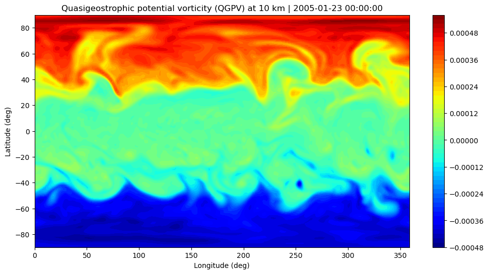
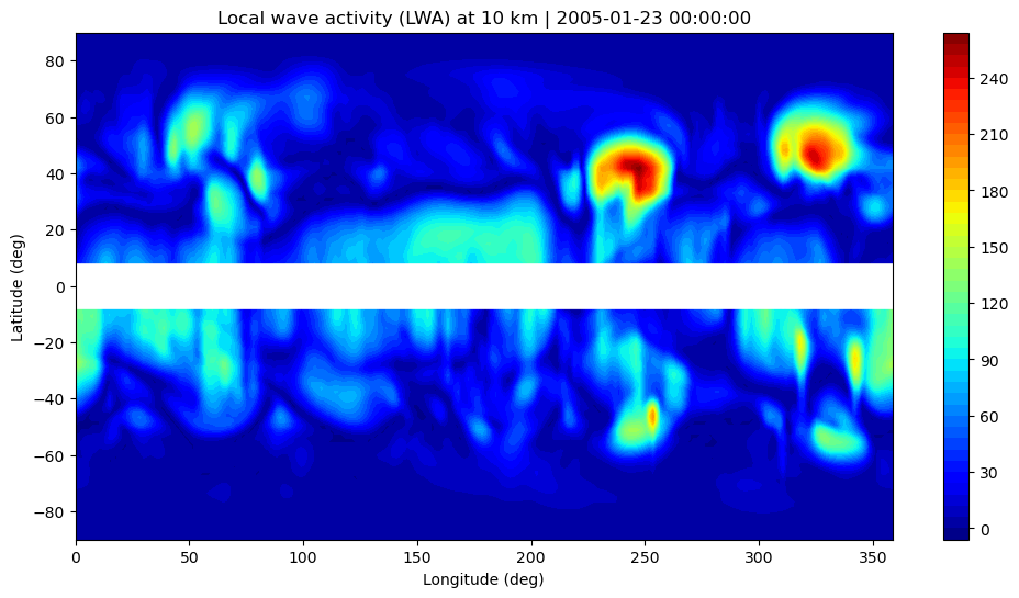
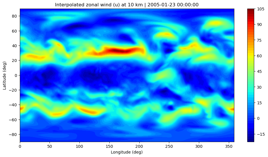
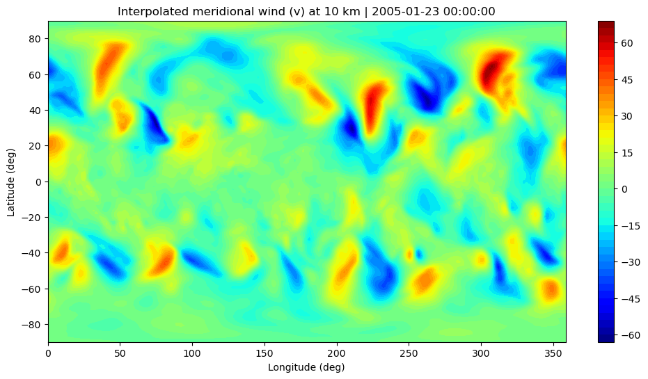
3D Variables on one pressure level to display
[5]:
variables_3d = [
    (selected_uvtinterp["qgpv"], 'Quasigeostrophic potential vorticity (QGPV)'),
    (selected_lwadiags["lwa"], 'Local wave activity (LWA)'),
    (selected_uvtinterp["interpolated_u"], 'Interpolated zonal wind (u)'),
    (selected_uvtinterp["interpolated_v"], 'Interpolated meridional wind (v)')
]

for variable, name in variables_3d:
    plt.figure(figsize=(12, 6))
    plt.contourf(variable['xlon'], variable['ylat'], variable, 50, cmap='jet')
    if name == 'Local wave activity (LWA)':
        plt.axhline(y=0, c='w', lw=30)
    plt.colorbar()
    plt.ylabel('Latitude (deg)')
    plt.xlabel('Longitude (deg)')
    plt.title(f"{name} at 10 km | {selected_time}")
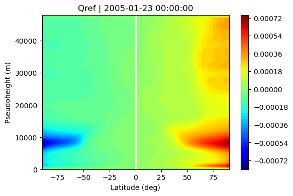
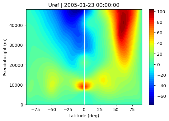
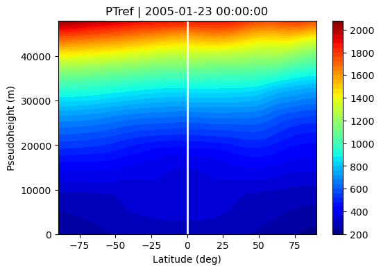
Reference states to be displayed on y-z plane
[6]:
variables_yz = [
    (selected_refstates["qref"], 'Qref'),
    (selected_refstates["uref"], 'Uref'),
    (selected_refstates["ptref"], 'PTref')
]

for variable, name in variables_yz:
    plt.figure(figsize=(6, 4))
    plt.contourf(variable['ylat'], variable['height'], variable, 50, cmap='jet')
    plt.axvline(x=0, c='w', lw=2)
    plt.xlabel('Latitude (deg)')
    plt.ylabel('Pseudoheight (m)')
    plt.colorbar()
    plt.title(f'{name} | {selected_time}')
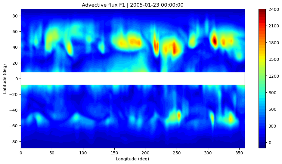
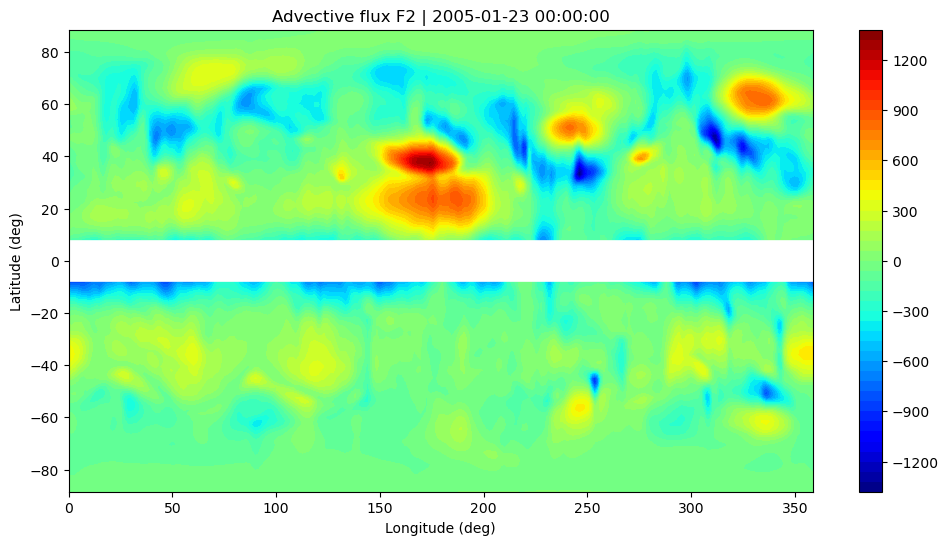
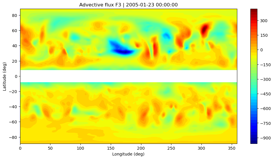
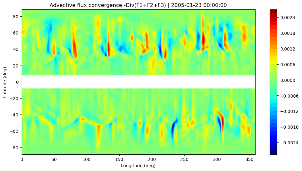
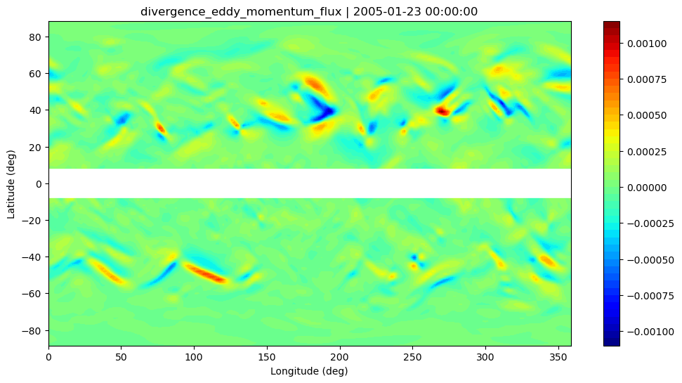
Vertically averaged variables to be displayed on x-y plane
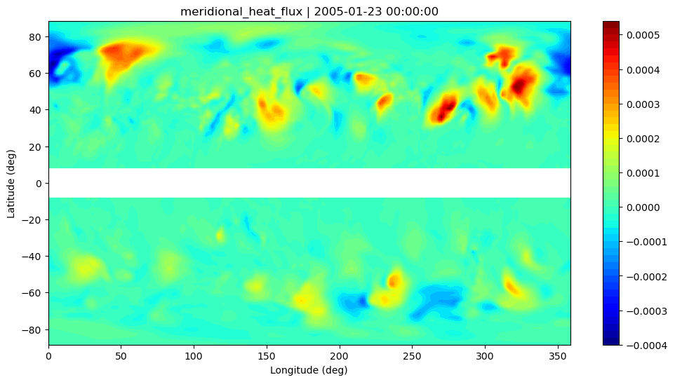
[7]:
variables_xy = [
    (selected_lwadiags["adv_flux_f1"], 'Advective flux F1'),
    (selected_lwadiags["adv_flux_f2"], 'Advective flux F2'),
    (selected_lwadiags["adv_flux_f3"], 'Advective flux F3'),
    (selected_lwadiags["convergence_zonal_advective_flux"], 'Advective flux convergence -Div(F1+F2+F3)'),
    (selected_lwadiags["divergence_eddy_momentum_flux"], 'divergence_eddy_momentum_flux'),
    (selected_lwadiags["meridional_heat_flux"], 'meridional_heat_flux')
]

for variable, name in variables_xy:
    plt.figure(figsize=(12, 6))
    plt.contourf(variable['xlon'], variable['ylat'][1:-1], variable[1:-1, :], 50, cmap='jet')
    plt.axhline(y=0, c='w', lw=30)
    plt.ylabel('Latitude (deg)')
    plt.xlabel('Longitude (deg)')
    plt.colorbar()
    plt.title(f'{name} | {selected_time}')
    plt.show()
Write to disk
Write with xarray’s `to_netcdf <https://docs.xarray.dev/en/stable/generated/xarray.Dataset.to_netcdf.html>`__.
[8]:
xr.merge([uvtinterp, refstates, lwadiags]).to_netcdf("2005-01-23_to_2005-01-30_output_xr.nc")
To reduce the file size, compression and/or integer-based value packing can be added by specifying an appropriate encoding for the variables.